AI applications can often start small in terms of compute, data, and monetary costs. As production applications scale due to increased user engagement, key factors such as the cost associated with storing and retrieving large volumes of data become critical optimization opportunities. These challenges can be addressed by focusing on:
Efficient Vector Search Algorithms
Automated Quantization Processes
Optimized Embedding Strategies
Both Retrieval-Augmented Generation (RAG) and agent-based systems rely on vector data—numerical representations of data objects like images, videos, and text—to perform semantic similarity searches. Systems that use RAG or agent-driven workflows must efficiently handle massive, high-dimensional data sets to maintain fast response times, minimize retrieval latency, and control infrastructure costs.
About the Tutorial
This tutorial equips you with the techniques needed to design, deploy, and manage advanced AI workloads at scale, ensuring optimal performance and cost efficiency.
Specifically, in this tutorial, you'll learn how to:
Generate embeddings using Voyage AI's
voyage-3-large, a general purpose, multilingual embedding model that is also quantization aware, and ingest them into a MongoDB database.Automatically quantize the embeddings to lower precision data types, optimizing both memory usage and query latency.
Run a query that compares float32, int8, and binary embeddings, weighing data type precision against efficiency and retrieval accuracy.
Measure the recall (also referred to as retention) of the quantized embeddings, which evaluates how effectively the quantized ANN search retrieves the same documents as a full-precision ENN search.
Note
Binary quantization is optimal for scenarios demanding reduced resource consumption, though it may require a rescoring pass to address any loss in accuracy.
Scalar quantization offers a practical middle ground, suitable for most use cases that need to balance performance and precision.
Float32 ensures maximum fidelity but has the steepest performance and memory overhead, making it less ideal for large-scale or latency-sensitive systems.
Prerequisites
To complete this tutorial, you must have the following:
Procedure
Import required libraries and set the environment variables.
Create an interactive Python notebook by saving a file with the
.ipynbextension.Install the libraries.
For this tutorial, you must import the following libraries:
pymongo
MongoDB Python driver to connect to the Atlas cluster, create indexes, and run queries.
voyageai
Voyage AI Python client to generate the embeddings for the data.
pandas
Data manipulation and analysis tool to load the data and prepare it for the vector search.
datasets
Hugging Face library that provides access to ready-made datasets.
matplotlib
Plotting and visualizing library to visualize the data.
To install the libraries, run the following:
pip install --quiet -U pymongo voyageai pandas datasets matplotlib Securely get and set environment variables.
The following
set_env_securelyhelper function gets and sets environment variables securely. Copy, paste, and run the following code and when prompted, set secret values such as your Voyage AI API key and Atlas cluster connection string.1 import getpass 2 import os 3 import voyageai 4 5 # Function to securely get and set environment variables 6 def set_env_securely(var_name, prompt): 7 value = getpass.getpass(prompt) 8 os.environ[var_name] = value 9 10 # Environment Variables 11 set_env_securely("VOYAGE_API_KEY", "Enter your Voyage API Key: ") 12 set_env_securely("MONGO_URI", "Enter your MongoDB URI: ") 13 MONGO_URI = os.environ.get("MONGO_URI") 14 if not MONGO_URI: 15 raise ValueError("MONGO_URI not set in environment variables.") 16 17 # Voyage Client 18 voyage_client = voyageai.Client()
Ingest the data into your Atlas cluster.
In this step, you load up to 250000 documents from the following datasets:
The wikipedia-22-12-en-voyage-embed
dataset contains Wikipedia article fragments with pre-generated
1024-dimensional float32 embeddings from Voyage AI's
voyage-3-large model. This is the primary document
collection with metadata. This dataset serves as a diverse
vector corpus for testing vector quantization effects in
semantic search. Each document in this dataset contains the
following fields:
| The ObjectId ( |
| The unique identifier for the document. |
| The title of the document. |
| The text of the document. |
| The URL of the document. |
| The wikipedia ID of the document. |
| The number of views of the document. |
| The paragraph ID in the document. |
| The number of languages in the document. |
| The 1024 dimensional vector embeddings for the document. |
The wikipedia-22-12-en-annotation dataset contains the annotated reference data for recall measurement function. This data is used as benchmark dataset for accuracy validation and to evaluate quantization impact on retrieval quality. Each document in this dataset contains the following fields, which are the ground truth used to evaluate the performance of the vector search:
| The ObjectId ( |
| The unique identifier for the document. |
| The wikipedia ID of the document. |
| The queries that contain the key phrases, questions, partial information, and sentences for the document. |
| The array of key phrases that are used to evaluate the performance of the vector search for the document. |
| The array of partial information that is used to evaluate the performance of the vector search for the document. |
| The array of questions that are used to evaluate the performance of the vector search for the document. |
| The array of sentences that are used to evaluate the performance of the vector search for the document. |
Define the functions to load the data into your cluster.
Copy, paste, and run the following code in your notebook. The sample code defines the following functions:
generate_bson_vectorto convert the embeddings in the dataset to BSON binary vectors for efficient storage and processing of your vectors.get_mongo_clientto get your Atlas cluster connection string.insert_dataframe_into_collectionto ingest data into the Atlas cluster.
1 import pandas as pd 2 from datasets import load_dataset 3 from bson.binary import Binary, BinaryVectorDtype 4 import pymongo 5 6 # Connect to Cluster 7 def get_mongo_client(uri): 8 """Connect to MongoDB and confirm the connection.""" 9 client = pymongo.MongoClient(uri) 10 if client.admin.command("ping").get("ok") == 1.0: 11 print("Connected to MongoDB successfully.") 12 return client 13 print("Failed to connect to MongoDB.") 14 return None 15 16 # Generate BSON Vector 17 def generate_bson_vector(array, data_type): 18 """Convert an array to BSON vector format.""" 19 array = [float(val) for val in eval(array)] 20 return Binary.from_vector(array, BinaryVectorDtype(data_type)) 21 22 # Load Datasets 23 def load_and_prepare_data(dataset_name, amount): 24 """Load and prepare streaming datasets for DataFrame.""" 25 data = load_dataset(dataset_name, streaming=True, split="train").take(amount) 26 return pd.DataFrame(data) 27 28 # Insert datasets into MongoDB Collection 29 def insert_dataframe_into_collection(df, collection): 30 """Insert Dataset records into MongoDB collection.""" 31 collection.insert_many(df.to_dict("records")) 32 print(f"Inserted {len(df)} records into '{collection.name}' collection.") Load the data into your cluster.
Copy, paste, and run the following code in your notebook to load the dataset into your Atlas cluster. This code performs the following actions:
Fetches the datasets.
Converts the embeddings to BSON format.
Creates collections in your Atlas cluster and inserts the data.
1 import pandas as pd 2 from bson.binary import Binary, BinaryVectorDtype 3 from pymongo.errors import CollectionInvalid 4 5 wikipedia_data_df = load_and_prepare_data("MongoDB/wikipedia-22-12-en-voyage-embed", amount=250000) 6 wikipedia_annotation_data_df = load_and_prepare_data("MongoDB/wikipedia-22-12-en-annotation", amount=250000) 7 wikipedia_annotation_data_df.drop(columns=["_id"], inplace=True) 8 9 # Convert embeddings to BSON format 10 wikipedia_data_df["embedding"] = wikipedia_data_df["embedding"].apply( 11 lambda x: generate_bson_vector(x, BinaryVectorDtype.FLOAT32) 12 ) 13 14 # MongoDB Setup 15 mongo_client = get_mongo_client(MONGO_URI) 16 DB_NAME = "testing_datasets" 17 db = mongo_client[DB_NAME] 18 19 collections = { 20 "wikipedia-22-12-en": wikipedia_data_df, 21 "wikipedia-22-12-en-annotation": wikipedia_annotation_data_df, 22 } 23 24 # Create Collections and Insert Data 25 for collection_name, df in collections.items(): 26 if collection_name not in db.list_collection_names(): 27 try: 28 db.create_collection(collection_name) 29 print(f"Collection '{collection_name}' created successfully.") 30 except CollectionInvalid: 31 print(f"Error creating collection '{collection_name}'.") 32 else: 33 print(f"Collection '{collection_name}' already exists.") 34 35 # Clear collection and insert fresh data 36 collection = db[collection_name] 37 collection.delete_many({}) 38 insert_dataframe_into_collection(df, collection) Connected to MongoDB successfully. Collection 'wikipedia-22-12-en' created successfully. Inserted 250000 records into 'wikipedia-22-12-en' collection. Collection 'wikipedia-22-12-en-annotation' created successfully. Inserted 87200 records into 'wikipedia-22-12-en-annotation' collection. Note
It might take some time to convert embeddings to BSON vectors and ingest the datasets into your Atlas cluster.
Verify that the datasets loaded successfully by logging into your Atlas cluster and visually inspecting the collections in Data Explorer.
Create Atlas Vector Search indexes on the collection.
In this step, you create the following three indexes on the embedding
field:
Scalar quantized Index | To use the scalar quantization method to quantize the embeddings. |
Binary quantized Index | To use the binary quantization method to quantize the embeddings. |
Float32 ANN Index | To use the float32 ANN method to quantize the embeddings. |
Define the function to create Atlas Vector Search index.
Copy, paste, and run the following in your notebook:
1 import time 2 from pymongo.operations import SearchIndexModel 3 4 def setup_vector_search_index(collection, index_definition, index_name="vector_index"): 5 new_vector_search_index_model = SearchIndexModel( 6 definition=index_definition, name=index_name, type="vectorSearch" 7 ) 8 9 # Create the new index 10 try: 11 result = collection.create_search_index(model=new_vector_search_index_model) 12 print(f"Creating index '{index_name}'...") 13 14 # Wait for initial sync to complete 15 print("Polling to check if the index is ready. This may take a couple of minutes.") 16 predicate=None 17 if predicate is None: 18 predicate = lambda index: index.get("queryable") is True 19 while True: 20 indices = list(collection.list_search_indexes(result)) 21 if len(indices) and predicate(indices[0]): 22 break 23 time.sleep(5) 24 print(f"Index '{index_name}' is ready for querying.") 25 return result 26 27 except Exception as e: 28 print(f"Error creating new vector search index '{index_name}': {e!s}") 29 return None Define the indexes.
The following index configurations implement a different quantization strategy:
vector_index_definition_scalar_quantizedThis configuration uses scalar quantization (int8), which:
Reduces each vector dimension from 32-bit float to 8-bit integer
Maintains a good balance between precision and memory efficiency
Is suitable for most production use cases where memory optimization is needed
vector_index_definition_binary_quantizedThis configuration uses binary quantization (int1), which:
Reduces each vector dimension to a single bit
Provides maximum memory efficiency
Is ideal for extremely large-scale deployments where memory constraints are critical
The automatic quantization happens transparently when these indexes are created, with Atlas Vector Search handling the conversion from float32 to the specified quantized format during index creation and search operations.
The
vector_index_definition_float32_annindex configuration indexes full fidelity vectors of1024dimensions by using thecosinesimilarity function.1 # Scalar Quantization 2 vector_index_definition_scalar_quantized = { 3 "fields": [ 4 { 5 "type": "vector", 6 "path": "embedding", 7 "quantization": "scalar", 8 "numDimensions": 1024, 9 "similarity": "cosine", 10 } 11 ] 12 } 13 # Binary Quantization 14 vector_index_definition_binary_quantized = { 15 "fields": [ 16 { 17 "type": "vector", 18 "path": "embedding", 19 "quantization": "binary", 20 "numDimensions": 1024, 21 "similarity": "cosine", 22 } 23 ] 24 } 25 # Float32 Embeddings 26 vector_index_definition_float32_ann = { 27 "fields": [ 28 { 29 "type": "vector", 30 "path": "embedding", 31 "numDimensions": 1024, 32 "similarity": "cosine", 33 } 34 ] 35 } Create the scalar, binary, and float32 indexes by using the
setup_vector_search_indexfunction.Set the collection and index names for the indexes.
wiki_data_collection = db["wikipedia-22-12-en"] wiki_annotation_data_collection = db["wikipedia-22-12-en-annotation"] vector_search_scalar_quantized_index_name = "vector_index_scalar_quantized" vector_search_binary_quantized_index_name = "vector_index_binary_quantized" vector_search_float32_ann_index_name = "vector_index_float32_ann" Create the Atlas Vector Search indexes.
1 setup_vector_search_index( 2 wiki_data_collection, 3 vector_index_definition_scalar_quantized, 4 vector_search_scalar_quantized_index_name, 5 ) 6 setup_vector_search_index( 7 wiki_data_collection, 8 vector_index_definition_binary_quantized, 9 vector_search_binary_quantized_index_name, 10 ) 11 setup_vector_search_index( 12 wiki_data_collection, 13 vector_index_definition_float32_ann, 14 vector_search_float32_ann_index_name, 15 ) Creating index 'vector_index_scalar_quantized'... Polling to check if the index is ready. This may take a couple of minutes. Index 'vector_index_scalar_quantized' is ready for querying. Creating index 'vector_index_binary_quantized'... Polling to check if the index is ready. This may take a couple of minutes. Index 'vector_index_binary_quantized' is ready for querying. Creating index 'vector_index_float32_ann'... Polling to check if the index is ready. This may take a couple of minutes. Index 'vector_index_float32_ann' is ready for querying. vector_index_float32_ann' Note
The operation might take a few minutes to complete. Indexes must be in Ready state to use them in queries.
Verify that the index creation succeeded by logging into your Atlas cluster and visually inspecting the indexes in Atlas Search.
Define the functions to generate embeddings and query a collection using the Atlas Vector Search indexes.
This code defines the following functions:
The
get_embeddingfunction generates 1024 dimension embeddings for the given text by using Voyage AI'svoyage-3-largeembedding model.The
custom_vector_searchfunction takes the following input parameters and returns the results of the vector search operation.user_queryQuery text string for which to generate embeddings.
collectionMongoDB collection to search.
embedding_pathField in the collection that contains the embeddings.
vector_search_index_nameName of index to use in the query.
top_kNumber of top documents in the results to return.
num_candidatesNumber of candidates to consider.
use_full_precisionFlag to perform ANN, if
False, or ENN, ifTrue, search.Note
The
use_full_precisionvalue is set toFalseby default for an ANN search. Set theuse_full_precisionvalue toTrueto perform an ENN search.Specifically, this function performs the following actions:
Generates the embeddings for the query text
Constructs the
$vectorSearchstageConfigures the type of search
Specifies the fields in the collection to return
Executes the pipeline after gathering performance statistics
Returns the results
1 def get_embedding(text, task_prefix="document"): 2 """Fetch embedding for a given text using Voyage AI.""" 3 if not text.strip(): 4 print("Empty text provided for embedding.") 5 return [] 6 result = voyage_client.embed([text], model="voyage-3-large", input_type=task_prefix) 7 return result.embeddings[0] 8 9 def custom_vector_search( 10 user_query, 11 collection, 12 embedding_path, 13 vector_search_index_name="vector_index", 14 top_k=5, 15 num_candidates=25, 16 use_full_precision=False, 17 ): 18 19 # Generate embedding for the user query 20 query_embedding = get_embedding(user_query, task_prefix="query") 21 22 if query_embedding is None: 23 return "Invalid query or embedding generation failed." 24 25 # Define the vector search stage 26 vector_search_stage = { 27 "$vectorSearch": { 28 "index": vector_search_index_name, 29 "queryVector": query_embedding, 30 "path": embedding_path, 31 "limit": top_k, 32 } 33 } 34 35 # Add numCandidates only for approximate search 36 if not use_full_precision: 37 vector_search_stage["$vectorSearch"]["numCandidates"] = num_candidates 38 else: 39 # Set exact to true for exact search using full precision float32 vectors and running exact search 40 vector_search_stage["$vectorSearch"]["exact"] = True 41 42 project_stage = { 43 "$project": { 44 "_id": 0, 45 "title": 1, 46 "text": 1, 47 "wiki_id": 1, 48 "url": 1, 49 "score": { 50 "$meta": "vectorSearchScore" 51 }, 52 } 53 } 54 55 # Define the aggregate pipeline with the vector search stage and additional stages 56 pipeline = [vector_search_stage, project_stage] 57 58 # Execute the explain command 59 explain_result = collection.database.command( 60 "explain", 61 {"aggregate": collection.name, "pipeline": pipeline, "cursor": {}}, 62 verbosity="executionStats", 63 ) 64 65 # Extract the execution time 66 vector_search_explain = explain_result["stages"][0]["$vectorSearch"] 67 execution_time_ms = vector_search_explain["explain"]["query"]["stats"]["context"][ 68 "millisElapsed" 69 ] 70 71 # Execute the actual query 72 results = list(collection.aggregate(pipeline)) 73 74 return {"results": results, "execution_time_ms": execution_time_ms}
Run an Atlas Vector Search query to evaluate the search performance.
The following query performs the vector searches across different quantization strategies, measuring performance metrics for scalar quantized, binary quantized, and full precision (float32) vectors while capturing latency measurements at each precision level and standardizing the result format for analytical comparison. It uses embeddings generated using Voyage AI for the query string "How do I increase my productivity for maximum output".
The query stores key essential performance indicators in the
results variable including precision level (Scalar, Binary,
Float32), result set size (top_k), query latency in
milliseconds, and retrieved document content, providing
comprehensive metrics for evaluating search performance across
different quantization strategies.
1 vector_search_indices = [ 2 vector_search_float32_ann_index_name, 3 vector_search_scalar_quantized_index_name, 4 vector_search_binary_quantized_index_name, 5 ] 6 7 # Random query 8 user_query = "How do I increase my productivity for maximum output" 9 test_top_k = 5 10 test_num_candidates = 25 11 12 # Result is a list of dictionaries with the following headings: precision, top_k, latency_ms, results 13 results = [] 14 15 for vector_search_index in vector_search_indices: 16 # Conduct a vector search operation using scalar quantized 17 vector_search_results = custom_vector_search( 18 user_query, 19 wiki_data_collection, 20 embedding_path="embedding", 21 vector_search_index_name=vector_search_index, 22 top_k=test_top_k, 23 num_candidates=test_num_candidates, 24 use_full_precision=False, 25 ) 26 # Include the precision in the results 27 precision = vector_search_index.split("vector_index")[1] 28 precision = precision.replace("quantized", "").capitalize() 29 30 results.append( 31 { 32 "precision": precision, 33 "top_k": test_top_k, 34 "num_candidates": test_num_candidates, 35 "latency_ms": vector_search_results["execution_time_ms"], 36 "results": vector_search_results["results"][0], # Just taking the first result, modify this to include more results if needed 37 } 38 ) 39 40 # Conduct a vector search operation using full precision 41 precision = "Float32_ENN" 42 vector_search_results = custom_vector_search( 43 user_query, 44 wiki_data_collection, 45 embedding_path="embedding", 46 vector_search_index_name="vector_index_scalar_quantized", 47 top_k=test_top_k, 48 num_candidates=test_num_candidates, 49 use_full_precision=True, 50 ) 51 52 results.append( 53 { 54 "precision": precision, 55 "top_k": test_top_k, 56 "num_candidates": test_num_candidates, 57 "latency_ms": vector_search_results["execution_time_ms"], 58 "results": vector_search_results["results"][0], # Just taking the first result, modify this to include more results if needed 59 } 60 ) 61 62 # Convert the results to a pandas DataFrame with the headings: precision, top_k, latency_ms 63 results_df = pd.DataFrame(results) 64 results_df.columns = ["precision", "top_k", "num_candidates", "latency_ms", "results"] 65 66 # To display the results: 67 results_df.head()
precision top_k num_candidates latency_ms results 0 _float32_ann 5 25 1659.498601 {'title': 'Henry Ford', 'text': 'Ford had deci... 1 _scalar_ 5 25 951.537687 {'title': 'Gross domestic product', 'text': 'F... 2 _binary_ 5 25 344.585193 {'title': 'Great Depression', 'text': 'The fir... 3 Float32_ENN 5 25 0.231693 {'title': 'Great Depression', 'text': 'The fir...
The performance metrics in the results show latency differences across precision levels. This demonstrates that while quantization provides substantial performance improvements, there's a clear trade-off between precision and retrieval speed, with full-precision float32 operations requiring notably more computational time compared to their quantized counterparts.
Measure latency with varying top-k and num_candidates values.
The following query introduces a systematic latency measurement
framewwork that evaluates vector search performance across
different precision levels and retrieval scales. The parameter
top-k not only determines the number of results to return but
also sets the numCandidates parameter in MongoDB's HNSW graph search.
The numCandidates value influences how many nodes in the
HNSW graph Atlas Vector Search
explores during the ANN search. Here, a higher value increases
the likelihood of finding the true nearest neighbors but requires
more computation time.
Define the function to format the
latency_msto a human-readable format.1 from datetime import timedelta 2 3 def format_time(ms): 4 """Convert milliseconds to a human-readable format""" 5 delta = timedelta(milliseconds=ms) 6 7 # Extract minutes, seconds, and milliseconds with more precision 8 minutes = delta.seconds // 60 9 seconds = delta.seconds % 60 10 milliseconds = round(ms % 1000, 3) # Keep 3 decimal places for milliseconds 11 12 # Format based on duration 13 if minutes > 0: 14 return f"{minutes}m {seconds}.{milliseconds:03.0f}s" 15 elif seconds > 0: 16 return f"{seconds}.{milliseconds:03.0f}s" 17 else: 18 return f"{milliseconds:.3f}ms" Define the function to measure the latency of the vector search query.
The following function takes a
user_query, acollection, avector_search_index_name, ause_full_precisionvalue, atop_k_valuesvalue, and anum_candidates_valuesvalue as input and returns the results of the vector search. Here, make a note of the following:The latency increases as the
top_kandnum_candidatesvalues increase because the vector search operation uses a larger number of documents and causes the search to take longer.The latency is higher for full fidelity search (
use_full_precision=True) than for approximate search (use_full_precision=False) because full fidelity search takes longer than approximate search as it searches the entire dataset, using the full precision float32 vectors.The latency of quantized search is lower than full fidelity search because the quantized search uses the approximate search and the quantized vectors.
1 def measure_latency_with_varying_topk( 2 user_query, 3 collection, 4 vector_search_index_name="vector_index_scalar_quantized", 5 use_full_precision=False, 6 top_k_values=[5, 10, 100], 7 num_candidates_values=[25, 50, 100, 200, 500, 1000, 2000, 5000, 10000], 8 ): 9 results_data = [] 10 11 # Conduct vector search operation for each (top_k, num_candidates) combination 12 for top_k in top_k_values: 13 for num_candidates in num_candidates_values: 14 # Skip scenarios where num_candidates < top_k 15 if num_candidates < top_k: 16 continue 17 18 # Construct the precision name 19 precision_name = vector_search_index_name.split("vector_index")[1] 20 precision_name = precision_name.replace("quantized", "").capitalize() 21 22 # If use_full_precision is true, then the precision name is "_float32_" 23 if use_full_precision: 24 precision_name = "_float32_ENN" 25 26 # Perform the vector search 27 vector_search_results = custom_vector_search( 28 user_query=user_query, 29 collection=collection, 30 embedding_path="embedding", 31 vector_search_index_name=vector_search_index_name, 32 top_k=top_k, 33 num_candidates=num_candidates, 34 use_full_precision=use_full_precision, 35 ) 36 37 # Extract the execution time (latency) 38 latency_ms = vector_search_results["execution_time_ms"] 39 40 # Store results 41 results_data.append( 42 { 43 "precision": precision_name, 44 "top_k": top_k, 45 "num_candidates": num_candidates, 46 "latency_ms": latency_ms, 47 } 48 ) 49 50 return results_data Run the Atlas Vector Search query to measure the latency.
The latency evaluation operation conducts a comprehensive performance analysis by executing searches across all quantization strategies, testing multiple result set sizes, capturing standardized performance metrics, and aggregating results for comparative analysis, enabling detailed evaluation of vector search behavior under different configurations and retrieval loads.
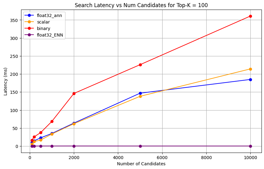
1 # Run the measurements 2 user_query = "How do I increase my productivity for maximum output" 3 top_k_values = [5, 10, 50, 100] 4 num_candidates_values = [25, 50, 100, 200, 500, 1000, 2000, 5000, 10000] 5 6 latency_results = [] 7 8 for vector_search_index in vector_search_indices: 9 latency_results.append( 10 measure_latency_with_varying_topk( 11 user_query, 12 wiki_data_collection, 13 vector_search_index_name=vector_search_index, 14 use_full_precision=False, 15 top_k_values=top_k_values, 16 num_candidates_values=num_candidates_values, 17 ) 18 ) 19 20 # Conduct vector search operation using full precision 21 latency_results.append( 22 measure_latency_with_varying_topk( 23 user_query, 24 wiki_data_collection, 25 vector_search_index_name="vector_index_scalar_quantized", 26 use_full_precision=True, 27 top_k_values=top_k_values, 28 num_candidates_values=num_candidates_values, 29 ) 30 ) 31 32 # Combine all results into a single DataFrame 33 all_latency_results = pd.concat([pd.DataFrame(latency_results)]) Top-K: 5, NumCandidates: 25, Latency: 1672.855906 ms, Precision: _float32_ann ... Top-K: 100, NumCandidates: 10000, Latency: 184.905389 ms, Precision: _float32_ann Top-K: 5, NumCandidates: 25, Latency: 828.45855 ms, Precision: _scalar_ ... Top-K: 100, NumCandidates: 10000, Latency: 214.199836 ms, Precision: _scalar_ Top-K: 5, NumCandidates: 25, Latency: 400.160243 ms, Precision: _binary_ ... Top-K: 100, NumCandidates: 10000, Latency: 360.908558 ms, Precision: _binary_ Top-K: 5, NumCandidates: 25, Latency: 0.239107 ms, Precision: _float32_ENN ... Top-K: 100, NumCandidates: 10000, Latency: 0.179203 ms, Precision: _float32_ENN The latency measurements reveal a clear performance hierarchy across precision types, where binary quantization demonstrates the fastest retrieval times, followed by scalar quantization. The full precision float32 ANN operations show significantly higher latencies. The performance gap between quantized and full precision searches become more pronounced as Top-K values increase. The float32 ENN operations are the slowest, but they provide the highest precision results.
Plot the search latency against various top-k values.
1 import matplotlib.pyplot as plt 2 3 # Map your precision field to the labels and colors you want in the legend 4 precision_label_map = { 5 "_scalar_": "scalar", 6 "_binary_": "binary", 7 "_float32_ann": "float32_ann", 8 "_float32_ENN": "float32_ENN", 9 } 10 11 precision_color_map = { 12 "_scalar_": "orange", 13 "_binary_": "red", 14 "_float32_ann": "blue", 15 "_float32_ENN": "purple", 16 } 17 18 # Flatten all measurements and find the unique top_k values 19 all_measurements = [m for precision_list in latency_results for m in precision_list] 20 unique_topk = sorted(set(m["top_k"] for m in all_measurements)) 21 22 # For each top_k, create a separate plot 23 for k in unique_topk: 24 plt.figure(figsize=(10, 6)) 25 26 # For each precision type, filter out measurements for the current top_k value 27 for measurements in latency_results: 28 # Filter measurements with top_k equal to the current k 29 filtered = [m for m in measurements if m["top_k"] == k] 30 if not filtered: 31 continue 32 33 # Extract x (num_candidates) and y (latency) values 34 x = [m["num_candidates"] for m in filtered] 35 y = [m["latency_ms"] for m in filtered] 36 37 # Determine the precision, label, and color from the first measurement in this filtered list 38 precision = filtered[0]["precision"] 39 label = precision_label_map.get(precision, precision) 40 color = precision_color_map.get(precision, "blue") 41 42 # Plot the line for this precision type 43 plt.plot(x, y, marker="o", color=color, label=label) 44 45 # Label axes and add title including the top_k value 46 plt.xlabel("Number of Candidates") 47 plt.ylabel("Latency (ms)") 48 plt.title(f"Search Latency vs Num Candidates for Top-K = {k}") 49 50 # Add a legend and grid, then show the plot 51 plt.legend() 52 plt.grid(True) 53 plt.show() The code returns the following latency charts, which illustrate how vector search document retrieval performs with different embedding precision types, binary, scalar, and float32, as the
top-k(the number of results retrieved) increases: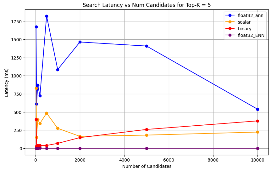 click to enlarge
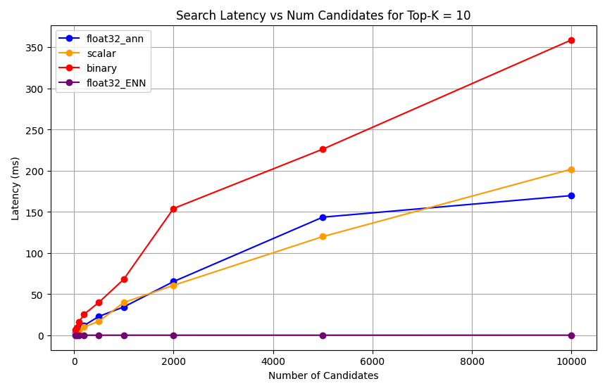 click to enlarge
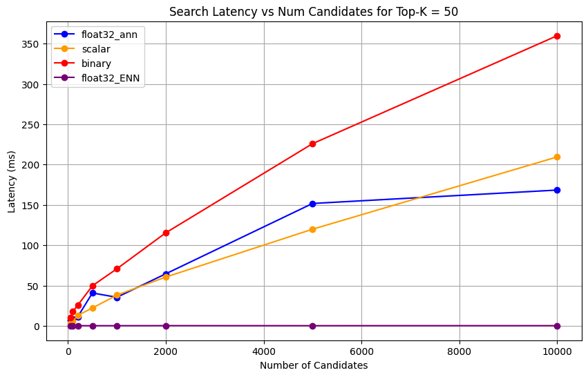 click to enlarge
Measure the representation capacity and retention.
The following query measures how effectively Atlas Vector Search retrieves relevant documents from the ground truth dataset. It is calculated as the ratio of correctly found relevant documents to the total number of relevant documents in the ground truth (Found/Total). For example, if a query has 5 relevant documents in the ground truth and Atlas Vector Search finds 4 of them, the recall would be 0.8 or 80%.
Define a function to measure the representational capacity and retention of the vector search operation. This function does the following:
Creates the baseline search using the full precision float32 vectors and ENN search.
Creates the quantized search using the quantized vectors and ANN search.
Computes the retention of the quantized search compared to the baseline search.
The retention must be maintained within a reasonable range for the quantized search. If the representational capacity is low, it means that the vector search operation is not able to capture the semantic meaning of the query and the results might not be accurate. This indicates that the quantization is not effective and the initial embedding model used is not effective for the quantization process. We recommend utilizing embedding models that are quantization aware, meaning that during the training process, the model is specifically optimized to produce embeddings that maintain their semantic properties even after quantization.
1 def measure_representational_capacity_retention_against_float_enn( 2 ground_truth_collection, 3 collection, 4 quantized_index_name, # This is used for both the quantized search and (with use_full_precision=True) for the baseline. 5 top_k_values, # List/array of top-k values to test. 6 num_candidates_values, # List/array of num_candidates values to test. 7 num_queries_to_test=1, 8 ): 9 retention_results = {"per_query_retention": {}} 10 overall_retention = {} # overall_retention[top_k][num_candidates] = [list of retention values] 11 12 # Initialize overall retention structure 13 for top_k in top_k_values: 14 overall_retention[top_k] = {} 15 for num_candidates in num_candidates_values: 16 if num_candidates < top_k: 17 continue 18 overall_retention[top_k][num_candidates] = [] 19 20 # Extract and store the precision name from the quantized index name. 21 precision_name = quantized_index_name.split("vector_index")[1] 22 precision_name = precision_name.replace("quantized", "").capitalize() 23 retention_results["precision_name"] = precision_name 24 retention_results["top_k_values"] = top_k_values 25 retention_results["num_candidates_values"] = num_candidates_values 26 27 # Load ground truth annotations 28 ground_truth_annotations = list( 29 ground_truth_collection.find().limit(num_queries_to_test) 30 ) 31 print(f"Loaded {len(ground_truth_annotations)} ground truth annotations") 32 33 # Process each ground truth annotation 34 for annotation in ground_truth_annotations: 35 # Use the ground truth wiki_id from the annotation. 36 ground_truth_wiki_id = annotation["wiki_id"] 37 38 # Process only queries that are questions. 39 for query_type, queries in annotation["queries"].items(): 40 if query_type.lower() not in ["question", "questions"]: 41 continue 42 43 for query in queries: 44 # Prepare nested dict for this query 45 if query not in retention_results["per_query_retention"]: 46 retention_results["per_query_retention"][query] = {} 47 48 # For each valid combination of top_k and num_candidates 49 for top_k in top_k_values: 50 if top_k not in retention_results["per_query_retention"][query]: 51 retention_results["per_query_retention"][query][top_k] = {} 52 for num_candidates in num_candidates_values: 53 if num_candidates < top_k: 54 continue 55 56 # Baseline search: full precision using ENN (Float32) 57 baseline_result = custom_vector_search( 58 user_query=query, 59 collection=collection, 60 embedding_path="embedding", 61 vector_search_index_name=quantized_index_name, 62 top_k=top_k, 63 num_candidates=num_candidates, 64 use_full_precision=True, 65 ) 66 baseline_ids = { 67 res["wiki_id"] for res in baseline_result["results"] 68 } 69 70 # Quantized search: 71 quantized_result = custom_vector_search( 72 user_query=query, 73 collection=collection, 74 embedding_path="embedding", 75 vector_search_index_name=quantized_index_name, 76 top_k=top_k, 77 num_candidates=num_candidates, 78 use_full_precision=False, 79 ) 80 quantized_ids = { 81 res["wiki_id"] for res in quantized_result["results"] 82 } 83 84 # Compute retention for this combination 85 if baseline_ids: 86 retention = len( 87 baseline_ids.intersection(quantized_ids) 88 ) / len(baseline_ids) 89 else: 90 retention = 0 91 92 # Store the results per query 93 retention_results["per_query_retention"][query].setdefault( 94 top_k, {} 95 )[num_candidates] = { 96 "ground_truth_wiki_id": ground_truth_wiki_id, 97 "baseline_ids": sorted(baseline_ids), 98 "quantized_ids": sorted(quantized_ids), 99 "retention": retention, 100 } 101 overall_retention[top_k][num_candidates].append(retention) 102 103 print( 104 f"Query: '{query}' | top_k: {top_k}, num_candidates: {num_candidates}" 105 ) 106 print(f" Ground Truth wiki_id: {ground_truth_wiki_id}") 107 print(f" Baseline IDs (Float32): {sorted(baseline_ids)}") 108 print( 109 f" Quantized IDs: {precision_name}: {sorted(quantized_ids)}" 110 ) 111 print(f" Retention: {retention:.4f}\n") 112 113 # Compute overall average retention per combination 114 avg_overall_retention = {} 115 for top_k, cand_dict in overall_retention.items(): 116 avg_overall_retention[top_k] = {} 117 for num_candidates, retentions in cand_dict.items(): 118 if retentions: 119 avg = sum(retentions) / len(retentions) 120 else: 121 avg = 0 122 avg_overall_retention[top_k][num_candidates] = avg 123 print( 124 f"Overall Average Retention for top_k {top_k}, num_candidates {num_candidates}: {avg:.4f}" 125 ) 126 127 retention_results["average_retention"] = avg_overall_retention 128 return retention_results Evaluate and compare the performance of your Atlas Vector Search indexes.
1 overall_recall_results = [] 2 top_k_values = [5, 10, 50, 100] 3 num_candidates_values = [25, 50, 100, 200, 500, 1000, 5000] 4 num_queries_to_test = 1 5 6 for vector_search_index in vector_search_indices: 7 overall_recall_results.append( 8 measure_representational_capacity_retention_against_float_enn( 9 ground_truth_collection=wiki_annotation_data_collection, 10 collection=wiki_data_collection, 11 quantized_index_name=vector_search_index, 12 top_k_values=top_k_values, 13 num_candidates_values=num_candidates_values, 14 num_queries_to_test=num_queries_to_test, 15 ) 16 ) Loaded 1 ground truth annotations Query: 'What happened in 2022?' | top_k: 5, num_candidates: 25 Ground Truth wiki_id: 69407798 Baseline IDs (Float32): [52251217, 60254944, 64483771, 69094871] Quantized IDs: _float32_ann: [60254944, 64483771, 69094871] Retention: 0.7500 ... Query: 'What happened in 2022?' | top_k: 5, num_candidates: 5000 Ground Truth wiki_id: 69407798 Baseline IDs (Float32): [52251217, 60254944, 64483771, 69094871] Quantized IDs: _float32_ann: [52251217, 60254944, 64483771, 69094871] Retention: 1.0000 Query: 'What happened in 2022?' | top_k: 10, num_candidates: 25 Ground Truth wiki_id: 69407798 Baseline IDs (Float32): [52251217, 60254944, 64483771, 69094871, 69265870] Quantized IDs: _float32_ann: [60254944, 64483771, 65225795, 69094871, 70149799] Retention: 1.0000 ... Query: 'What happened in 2022?' | top_k: 10, num_candidates: 5000 Ground Truth wiki_id: 69407798 Baseline IDs (Float32): [52251217, 60254944, 64483771, 69094871, 69265870] Quantized IDs: _float32_ann: [52251217, 60254944, 64483771, 69094871, 69265870] Retention: 1.0000 Query: 'What happened in 2022?' | top_k: 50, num_candidates: 50 Ground Truth wiki_id: 69407798 Baseline IDs (Float32): [25391, 832774, 8351234, 18426568, 29868391, 52241897, 52251217, 60254944, 63422045, 64483771, 65225795, 69094871, 69265859, 69265870, 70149799, 70157964] Quantized IDs: _float32_ann: [25391, 8351234, 29868391, 40365067, 52241897, 52251217, 60254944, 64483771, 65225795, 69094871, 69265859, 69265870, 70149799, 70157964] Retention: 0.8125 ... Query: 'What happened in 2022?' | top_k: 50, num_candidates: 5000 Ground Truth wiki_id: 69407798 Baseline IDs (Float32): [25391, 832774, 8351234, 18426568, 29868391, 52241897, 52251217, 60254944, 63422045, 64483771, 65225795, 69094871, 69265859, 69265870, 70149799, 70157964] Quantized IDs: _float32_ann: [25391, 832774, 8351234, 18426568, 29868391, 52241897, 52251217, 60254944, 63422045, 64483771, 65225795, 69094871, 69265859, 69265870, 70149799, 70157964] Retention: 1.0000 Query: 'What happened in 2022?' | top_k: 100, num_candidates: 100 Ground Truth wiki_id: 69407798 Baseline IDs (Float32): [16642, 22576, 25391, 547384, 737930, 751099, 832774, 8351234, 17742072, 18426568, 29868391, 40365067, 52241897, 52251217, 52851695, 53992315, 57798792, 60163783, 60254944, 62750956, 63422045, 64483771, 65225795, 65593860, 69094871, 69265859, 69265870, 70149799, 70157964] Quantized IDs: _float32_ann: [22576, 25391, 243401, 547384, 751099, 8351234, 17742072, 18426568, 29868391, 40365067, 47747350, 52241897, 52251217, 52851695, 53992315, 57798792, 60254944, 64483771, 65225795, 69094871, 69265859, 69265870, 70149799, 70157964] Retention: 0.7586 ... Query: 'What happened in 2022?' | top_k: 100, num_candidates: 5000 Ground Truth wiki_id: 69407798 Baseline IDs (Float32): [16642, 22576, 25391, 547384, 737930, 751099, 832774, 8351234, 17742072, 18426568, 29868391, 40365067, 52241897, 52251217, 52851695, 53992315, 57798792, 60163783, 60254944, 62750956, 63422045, 64483771, 65225795, 65593860, 69094871, 69265859, 69265870, 70149799, 70157964] Quantized IDs: _float32_ann: [16642, 22576, 25391, 547384, 737930, 751099, 832774, 8351234, 17742072, 18426568, 29868391, 40365067, 52241897, 52251217, 52851695, 53992315, 57798792, 60163783, 60254944, 62750956, 63422045, 64483771, 65225795, 65593860, 69094871, 69265859, 69265870, 70149799, 70157964] Retention: 1.0000 Overall Average Retention for top_k 5, num_candidates 25: 0.7500 ... The output shows the retention results for each query in the ground truth dataset. The retention is expressed as a decimal between 0 and 1 where 1.0 means that the ground truth IDs are retained and 0.25 means only 25% of the ground truth IDs are retained.
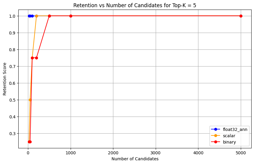
Plot the retention capability of the different precision types.
1 import matplotlib.pyplot as plt 2 3 # Define colors and labels for each precision type 4 precision_colors = {"_scalar_": "orange", "_binary_": "red", "_float32_": "green"} 5 6 if overall_recall_results: 7 # Determine unique top_k values from the first result's average_retention keys 8 unique_topk = sorted(list(overall_recall_results[0]["average_retention"].keys())) 9 10 for k in unique_topk: 11 plt.figure(figsize=(10, 6)) 12 # For each precision type, plot retention vs. number of candidates at this top_k 13 for result in overall_recall_results: 14 precision_name = result.get("precision_name", "unknown") 15 color = precision_colors.get(precision_name, "blue") 16 # Get candidate values from the average_retention dictionary for top_k k 17 candidate_values = sorted(result["average_retention"][k].keys()) 18 retention_values = [ 19 result["average_retention"][k][nc] for nc in candidate_values 20 ] 21 22 plt.plot( 23 candidate_values, 24 retention_values, 25 marker="o", 26 label=precision_name.strip("_"), 27 color=color, 28 ) 29 30 plt.xlabel("Number of Candidates") 31 plt.ylabel("Retention Score") 32 plt.title(f"Retention vs Number of Candidates for Top-K = {k}") 33 plt.legend() 34 plt.grid(True) 35 plt.show() 36 37 # Print detailed average retention results 38 print("\nDetailed Average Retention Results:") 39 for result in overall_recall_results: 40 precision_name = result.get("precision_name", "unknown") 41 print(f"\n{precision_name} Embedding:") 42 for k in sorted(result["average_retention"].keys()): 43 print(f"\nTop-K: {k}") 44 for nc in sorted(result["average_retention"][k].keys()): 45 ret = result["average_retention"][k][nc] 46 print(f" NumCandidates: {nc}, Retention: {ret:.4f}") The code returns the retention charts for the following:
 click to enlarge
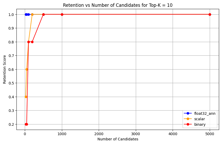 click to enlarge
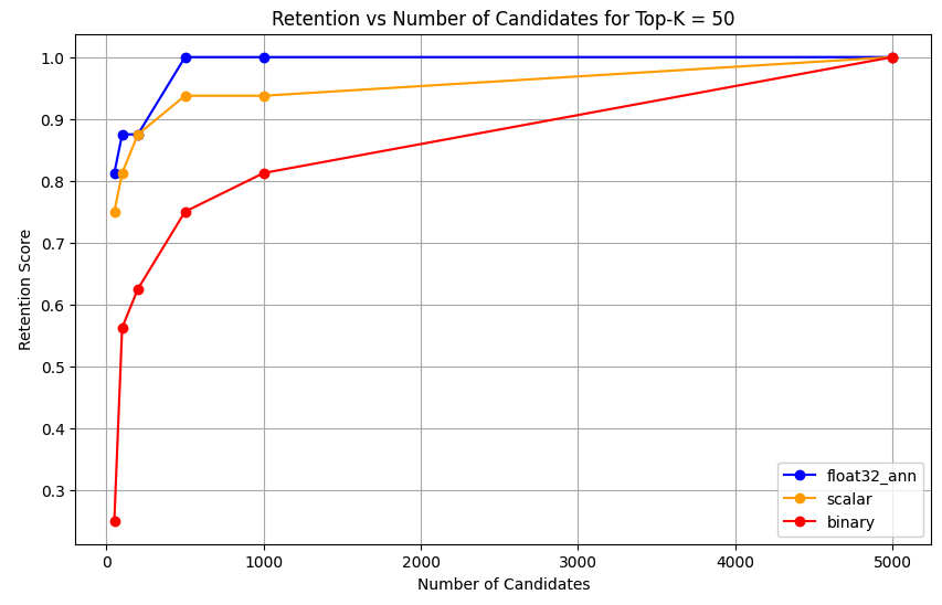 click to enlarge
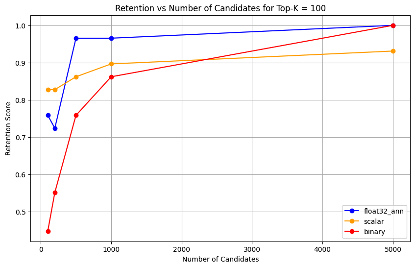 click to enlarge
For
float32_ann,scalar, andbinaryembeddings, the code also returns detailed average retention results similar to the following:Detailed Average Retention Results: _float32_ann Embedding: Top-K: 5 NumCandidates: 25, Retention: 1.0000 NumCandidates: 50, Retention: 1.0000 NumCandidates: 100, Retention: 1.0000 NumCandidates: 200, Retention: 1.0000 NumCandidates: 500, Retention: 1.0000 NumCandidates: 1000, Retention: 1.0000 NumCandidates: 5000, Retention: 1.0000 Top-K: 10 NumCandidates: 25, Retention: 1.0000 NumCandidates: 50, Retention: 1.0000 NumCandidates: 100, Retention: 1.0000 NumCandidates: 200, Retention: 1.0000 NumCandidates: 500, Retention: 1.0000 NumCandidates: 1000, Retention: 1.0000 NumCandidates: 5000, Retention: 1.0000 Top-K: 50 NumCandidates: 50, Retention: 0.8125 NumCandidates: 100, Retention: 0.8750 NumCandidates: 200, Retention: 0.8750 NumCandidates: 500, Retention: 1.0000 NumCandidates: 1000, Retention: 1.0000 NumCandidates: 5000, Retention: 1.0000 Top-K: 100 NumCandidates: 100, Retention: 0.7586 NumCandidates: 200, Retention: 0.7241 NumCandidates: 500, Retention: 0.9655 NumCandidates: 1000, Retention: 0.9655 NumCandidates: 5000, Retention: 1.0000 _scalar_ Embedding: Top-K: 5 NumCandidates: 25, Retention: 0.2500 NumCandidates: 50, Retention: 0.5000 NumCandidates: 100, Retention: 0.7500 NumCandidates: 200, Retention: 1.0000 NumCandidates: 500, Retention: 1.0000 NumCandidates: 1000, Retention: 1.0000 NumCandidates: 5000, Retention: 1.0000 Top-K: 10 NumCandidates: 25, Retention: 0.4000 NumCandidates: 50, Retention: 0.6000 NumCandidates: 100, Retention: 0.8000 NumCandidates: 200, Retention: 1.0000 NumCandidates: 500, Retention: 1.0000 NumCandidates: 1000, Retention: 1.0000 NumCandidates: 5000, Retention: 1.0000 Top-K: 50 NumCandidates: 50, Retention: 0.7500 NumCandidates: 100, Retention: 0.8125 NumCandidates: 200, Retention: 0.8750 NumCandidates: 500, Retention: 0.9375 NumCandidates: 1000, Retention: 0.9375 NumCandidates: 5000, Retention: 1.0000 Top-K: 100 NumCandidates: 100, Retention: 0.8276 NumCandidates: 200, Retention: 0.8276 NumCandidates: 500, Retention: 0.8621 NumCandidates: 1000, Retention: 0.8966 NumCandidates: 5000, Retention: 0.9310 _binary_ Embedding: Top-K: 5 NumCandidates: 25, Retention: 0.2500 NumCandidates: 50, Retention: 0.2500 NumCandidates: 100, Retention: 0.7500 NumCandidates: 200, Retention: 0.7500 NumCandidates: 500, Retention: 1.0000 NumCandidates: 1000, Retention: 1.0000 NumCandidates: 5000, Retention: 1.0000 Top-K: 10 NumCandidates: 25, Retention: 0.2000 NumCandidates: 50, Retention: 0.2000 NumCandidates: 100, Retention: 0.8000 NumCandidates: 200, Retention: 0.8000 NumCandidates: 500, Retention: 1.0000 NumCandidates: 1000, Retention: 1.0000 NumCandidates: 5000, Retention: 1.0000 Top-K: 50 NumCandidates: 50, Retention: 0.2500 NumCandidates: 100, Retention: 0.5625 NumCandidates: 200, Retention: 0.6250 NumCandidates: 500, Retention: 0.7500 NumCandidates: 1000, Retention: 0.8125 NumCandidates: 5000, Retention: 1.0000 Top-K: 100 NumCandidates: 100, Retention: 0.4483 NumCandidates: 200, Retention: 0.5517 NumCandidates: 500, Retention: 0.7586 NumCandidates: 1000, Retention: 0.8621 NumCandidates: 5000, Retention: 1.0000 The recall results demonstrate distinct performance patterns across the three embedding types.
Scalar quantization shows a steady improvement indicating strong retrieval accuracy at higher K values. Binary quantization, while starting lower, improves at Top-K 50 and 100, suggesting a trade-off between computational efficiency and recall performance. Float32 embeddings demonstrate the strongest initial performance and reaching the same maximum recall as scalar quantization at Top-K 50 and 100.
This suggests that while float32 provides better recall at lower Top-K values, scalar quantization can achieve equivalent performance at higher Top-K values while offering improved computational efficiency. The binary quantization, despite its lower recall ceiling, might still be valuable in scenarios where memory and computational constraints outweigh the need for maximum recall accuracy.